Introduction
Algorithm
- DCT
- Coefficient Quantization
- Lossless Compression
Color
FutureThe Discrete Cosine Transform (DCT)
The key to the JPEG baseline compression process is a mathematical transformation known
as the Discrete Cosine Transform (DCT). The DCT is in a class of mathematical operations
that includes the well known Fast Fourier Transform (FFT), as well as many others. The
basic purpose of these operations is to take a signal and transform it from one type of
representation to another. For example, an image is a two-dimensional signal that is
perceived by the human visual system. The DCT can be used to convert the signal (spatial
information) into numeric data ("frequency" or "spectral" information)
so that the image’s information exists in a quantitative form that can be manipulated
for compression.
The signal for a graphical image can be thought of as a three-dimensional signal. The X
and Y-axes of the image’s signal are the two dimensions of the screen, while the
amplitude of the signal, the Z-axis, is the value of the pixel at (X, Y). This can be
represented visually by a two-dimensional array where each cell contains the numerical
value of the pixel at that location. As the specifics of a two-dimensional DCT matrix are
rather complex, we will simplify the problem by first considering the derivation and
intentions of a one-dimensional DCT matrix.
The One-Dimensional DCT
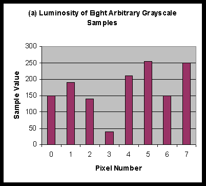 We start with a set of eight arbitrary
grayscale samples as charted below, where each bar represents the luminosity of a single
pixel.
We start with a set of eight arbitrary
grayscale samples as charted below, where each bar represents the luminosity of a single
pixel.
These values contain all the information necessary to define the eight pixels. Thus the
ultimate goal is to compress this data so it can be stored or transmitted and later
decompressed to reform the original image. However, as explained above, simple entropy or
statistical encoding of this data will not be extremely effective because in continuous
tone images, the levels of luminosity have equal probabilities of occurring. As a more
effective alternative, the DCT can manipulate this data, separating information crucial to
the definition of the image from information that’s presence is not perceivable by
the human eye. The insignificant information can then be "discarded" through the
quantization phase of JPEG coding, thus achieving large-scale compression. Simply put, the
purpose of the DCT transformation phase is to identify "pieces of information
in the image’s signal that can be effectively ‘thrown away’ without
seriously compromising the quality of the image" (Nelson 359). No information is
lost, nor is any compression achieved, in the DCT stage. This initial phase is merely a
preparatory step that allows for and leads to the lossy coefficient quantization stage
that follows.
The first step involved in the "rearrangement" of the data displayed in
figure (a) is to perform a level shift by 128, the result of which is shown in figure (b)
below.
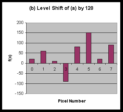
The samples have values in the range of 0 to 255. By shifting the level of their graph
by 128, half their range, we obtain the values of f(x) in figure (b). Using f(x), we can
decompose the eight sample values into a set of waveforms of different spatial
frequencies. This decomposition is where the separation of the more significant
low-frequency components from the less significant high-frequency components takes place.
Below is a set of waveforms of eight different spatial frequencies, all of uniform
amplitude and each sampled at eight points.
Below is a set of cosine waveforms of eight different spatial frequencies. 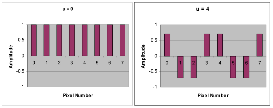
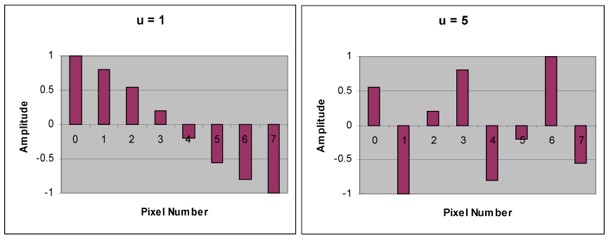
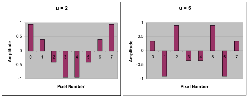
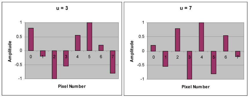
The top left waveform (u = 0) is simply a constant, whereas the other seven waveforms
(u = 1, …, 7) show an alternating behavior at progressively higher frequencies. These
waveforms, which are called cosine basis functions, are independent, meaning that there is
no way that a given waveform can be represented by any combination of the other waveforms.
However, the complete set of eight waveforms, when scaled by numbers called coefficients
and added together, can be used to represent any eight sample values such as those in
figure (b). The intention is to use the Discrete Cosine Transform to determine the values
of the coefficients. The coefficients plotted in figure (c) below are the output of an
8-point DCT for the eight sample values in figure (b).
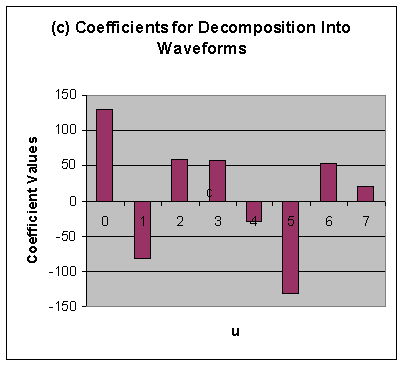
There is a direct correlation between the magnitude of the coefficient for a given
waveform and the impact of that particular waveform on the quality of the picture. The
coefficient that scales the constant basis function (u = 0) is called the DC coefficient,
while the other coefficients are called AC coefficients. Note that the DC term gives the
average over the set of samples. Furthermore, the DC term is usually a great deal larger
in magnitude than the AC terms, and, though it may not be evident in the small sampling
depicted by figure (c), as the elements move farther away from the DC term, they tend to
become lower and lower in value. Recall that the AC terms farther away from the DC term
represent coefficients of waveforms of greater spatial frequencies. The fact that these
coefficients tend to be smaller in magnitude suggests that higher-frequency image
components play a relatively small role in the determining picture quality, while the
majority of image definition comes from lower-frequency image components. This idea
becomes extremely important when applied two-dimensionally to an image, for JPEG exploits
this exact concept when deciding what information can be eliminated to achieve
compression.
The Two-Dimensional DCT
The one-dimensional DCT described above can be extended to apply to two-dimensional
image arrays. The two-dimensional cosine basis functions from which sample waveforms are
composed are created by multiplying a horizontally oriented set of one-dimensional 8-point
basis functions by a vertically oriented set of the same functions. It logically follows
that the horizontally oriented set of basis functions represents horizontal frequencies
and the other set of basis functions represents vertical frequencies.
By convention, the DC term of the horizontal basis functions is to the left, and the DC
term for the vertical basis functions is at the top. Consequently, the top, left element
of a two-dimensional DCT matrix contains a value that is almost always of a very great
magnitude. Furthermore, mirroring the trend found in a one-dimensional DCT matrix, the
farther away an AC term is from the DC term, the higher the frequency its corresponding
waveform will have and the smaller its magnitude will be. Although the concept of the
two-dimensional DCT is not as easily pictured using histograms as is the one-dimensional
DCT, the two-dimensional version employs the same underlying principles and thus can be
interpreted using identical reasoning (Pennebaker 33).
The actual formula for the two-dimensional DCT is shown below. The DCT is performed on
an N x N square matrix of pixel values, and it yields an N x N square matrix of frequency
coefficients. (In practice, N most often equals 8 because a larger block, though would
probably give better compression, often takes a great deal of time to perform DCT
calculations, creating an unreasonable tradeoff. As a result, DCT implementations
typically break the image down into more manageable 8 x 8 blocks.) The DCT formula looks
somewhat intimidating at first glance but can be implemented with a relatively
straightforward piece of code.
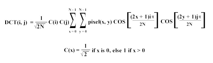
When writing code to implement this function, simple table lookups can replace several
terms of the equation to simplify the appearance of the algorithm. The two cosine terms
only need to be calculated once at the beginning of the program, and they can be stored
for later use. Likewise, the C(x) terms can also be replaced with table lookups. Code to
compute the DCT matrix for an N-by-N portion of a display looks somewhat like the
following (adapted from The Data Compression Book by Mark Nelson).