![]()
![]()
![]()
![]()
![]()
![]()
![]()
![]()
![]()
![]()
![]()
![]()
![]()
![]()
![]()
ALGORITHMS - A*
Algorithm A* is a best-first search algorithm that relies
on an open list and a closed list to find a path that is both optimal and
complete towards the goal. It works by combining the benefits of the uniform-cost
search and greedy search algorithms. A* makes use of both elements
by including two separate path finding functions in its algorithm that take
into account the cost from the root node to the current node and estimates
the path cost from the current node to the goal node.
The first function is g(n), which calculates the path cost between the start node and the current node. The second function is h(n), which is a heuristic to calculate the estimated path cost from the current node to the goal node. F(n) = g(n) + h(n). It represents the path cost of the most efficient estimated path towards the goal. A* continues to re-evaluate both g(n) and h(n) throughout the search for all of the nodes that it encounters in order to arrive at the minimal cost path to the goal. This algorithm is extremely popular for pathfinding in strategy computer games.
The process for A* is basically this:
1. Create an open list and a closed list that are both empty.
Put the start node in the open list.
2. Loop this until the goal is found or the open list is empty:
a. Find the node with the lowest F cost in the open list and place it in
the closed list.
b. Expand this node and for the adjacent nodes to this node:
i. If they are on the closed list, ignore.
ii. If not on the open list, add to open list, store the current node as
the parent for this adjacent node, and calculate the F,G, H costs of the
adjacent node.
iii. If on the open list, compare the G costs of this path to the node and
the old path to the node. If the G cost of using the current node to get
to the node is the lower cost, change the parent node of the adjacent node
to the current node. Recalculate F,G,H costs of the node.
3. If open list is empty, fail.
The terms locally finite, admissible, and monotonic all aid in the understanding of when A* can be expected to be complete, meaning that it finds a solution, and optimal, meaning that it finds the solution with the lowest path cost. A locally finite graph is one where none of the nodes on the graph have an infinite branching factor, thus none of the node paths branch forever. A branching factor of a node refers to the amount of new nodes that can be expanded from that node.
A heuristic is admissible if it is always optimistic; it either underestimates the path cost to the goal or provides a correct estimate for the path cost to the goal, but it never overestimates the path cost to the goal.
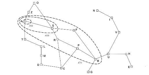
A heuristic is monotonic if in every path from the root to the goal the total estimated path cost does not decrease as the heuristic goes down a node tree. (illustration) Nonmonotonic heuristics can be made monotonic by the pathmax equation, which compares the estimated path cost of a node with the estimated path cost of its parent node. It then uses the higher path cost for estimation. Therefore, if the heuristic's estimated path cost decreases from one node to its child node, the pathmax equation uses the path cost of the parent node so that it is not evaluated as decreasing.
|
|
Fig.1 Illustration of a map featuring monoticity with contours at 380, 400 and 420.
A* is complete and optimal on graphs that are locally finite where the heuristics are admissible and monotonic.
A* must be locally finite, because if there exist an infinite amount of nodes where the estimated path cost, f(n), is less than the actual goal path cost then the algorithm could continue to explore these nodes without end, and it will be neither complete nor optimal.
How does monotocity affect A*'s completeness? Because A* is monotonic, the path cost increases as the node gets further from the root. Contours can be drawn to show areas where the estimated path cost, the f(n), for the nodes inside the areas are lower than or equal to the path cost for the outer bounds of the contours. These contours can be drawn as larger and larger areas that increase outwards as the f(n) for the outer bound of these contours increases. The first solution found is optimal since it is the first band where the f(n) for the contour is equal to the path cost for the goal. All the contours outside of this solution will have a higher f cost.
A*'s optimality is proved by contradiction. First, it is assumed that g is an optimal goal state with a path cost of f(g), that s is a suboptimal goal state with a path cost of g(s) > f(g), and that n is a node on an optimal path to g. We are assuming that A* selects s (the suboptimal goal) instead of n (the node on the optimal path) from the open list.
Since h is admissible, (optimistic), f(g) >= f(n). (The actual path cost is greater than or equal to the path cost estimated by the heuristic at n.)
If n is not chosen over s for expansion by A*, f(n) >= f(s). (The heuristic chooses the node with the lowest estimated F path cost.)
Thus, f(g) >= f(s).
Since s is a goal state, h(s) = 0. (The estimation from the
current node to the final node must be 0.)
So f(s) = g(s). (f(s) = g(s) + h(s).)
Thus, f(g) >= g(s). This contradicts the statement that
S is suboptimal so it must be true that A* never chooses a suboptimal path.
Since A* only can have as a solution a node that it has selected for expansion,
it is optimal.