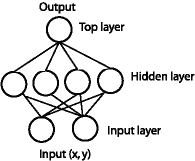
(Fig.1) A feed-forward network.

Feed-forward networks have the following characteristics:

1.	Perceptrons are arranged in layers, with the first layer taking in inputs and the last layer producing outputs. The middle layers have no connection with the external world, and hence are called hidden layers.
2.	Each perceptron in one layer is connected to every perceptron on the next layer. Hence information is constantly "fed forward" from one layer to the next., and this explains why these networks are called feed-forward networks.
3.	There is no connection among perceptrons in the same layer.

What's so cool about feed-forward networks?

Recall that a single perceptron can classify points into two regions that are linearly separable. Now let us extend the discussion into the separation of points into two regions that are not linearly separable. Consider the following network:

(Fig.2) A feed-forward network with one hidden layer.

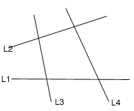
The same (x, y) is fed into the network through the perceptrons in the input layer. With four perceptrons that are independent of each other in the hidden layer, the point is classified into 4 pairs of linearly separable regions, each of which has a unique line separating the region.

(Fig.3) 4 lines each dividing the plane into 2 linearly separable regions.

The top perceptron performs logical operations on the outputs of the hidden layers so that the whole network classifies input points in 2 regions that might not be linearly separable. For instance, using the AND operator on these four outputs, one gets the intersection of the 4 regions that forms the center region.

(Fig.4) Intersection of 4 linearly separable regions forms the center region.

By varying the number of nodes in the hidden layer, the number of layers, and the number of input and output nodes, one can classification of points in arbitrary dimension into an arbitrary number of groups. Hence feed-forward networks are commonly used for classification.

Backpropagation -- learning in feed-forward networks:

Learning in feed-forward networks belongs to the realm of supervised learning, in which pairs of input and output values are fed into the network for many cycles, so that the network 'learns' the relationship between the input and output.

We provide the network with a number of training samples, which consists of an input vector i and its desired output o. For instance, in the classification problem, suppose we have points (1, 2) and (1, 3) belonging to group 0, points (2, 3) and (3, 4) belonging to group 1, (5, 6) and (6, 7) belonging to group 2, then for a feed-forward network with 2 input nodes and 2 output nodes, the training set would be:

{	i = (1, 2) , o =( 0, 0)
	i = (1, 3) , o = (0, 0)
	i = (2, 3) , o = (1, 0)
	i = (3, 4) , o = (1, 0)
	i = (5, 6) , o = (0, 1)
	i = (6, 7) , o = (0, 1) }

The basic rule for choosing the number of output nodes depends on the number of different regions. It is advisable to use a unary notation to represent the different regions, i.e. for each output only one node can have value 1. Hence the number of output nodes = number of different regions -1.

In backpropagation learning, every time an input vector of a training sample is presented, the output vector o is compared to the desired value d.

The comparison is done by calculating the squared difference of the two:

The value of Err tells us how far away we are from the desired value for a particular input. The goal of backpropagation is to minimize the sum of Err for all the training samples, so that the network behaves in the most "desirable" way.

Minimize

We can express Err in terms of the input vector (i), the weight vectors (w), and the threshold function of the perceptions. Using a continuous function (instead of the step function) as the threshold function, we can express the gradient of Err with respect to the w in terms of w and i.

Given the fact that decreasing the value of w in the direction of the gradient leads to the most rapid decrease in Err, we update the weight vectors every time a sample is presented using the following formula:

where n is the learning rate (a small number ~ 0.1)

Using this algorithm, the weight vectors are modified so that the value of Err for a particular input sample decreases a little bit every time the sample is presented. When all the samples are presented in turns for many cycles, the sum of Err gradually decreases to a minimum value, which is our goal as mentioned above.

Back to Architecture