Motion Planning in Robotics

        From the moment we wake up in the morning until our head hits the pillow at night, we must plan our actions.  Planning includes choosing the day's outfit based on the weather forecast, figuring out what to eat for breakfast, deciding the best route to work after listening to the traffic reports, and making a schedule of activities for the day.  Planning also occurs on another more instinctual level and includes decisions that we may take for granted, such as choosing to walk around a piece of furniture rather than climb over it in order to get to the door and deciding to take as straight and direct a path as possible rather than meander in circles when trying to reach a destination.  A large problem in the development of autonomous robots is devising a way to give them the capabilities to make their own plans in a variety of situations.  Motion planning refers to the computational process of moving from one place to another in the presence of obstacles.
        The degree of difficulty of motion planning in robots varies greatly depending on a couple of factors: whether all information regarding the obstacles (i.e. sizes, locations, motions, etc.) is known before the robot moves and whether these obstacles move around or stay in place as the robot moves.  The different possible scenarios are shown in the following chart:
 

    The simplest scenario, and therefore the most researched and understood one, is Case I.  In Case I, all obstacles are fixed in their positions, and all details about these obstacles are known before path planning takes place.  The problem for the robot, which is known as the basic motion planning problem, can be informally stated as getting from a starting point to an ending point without colliding with any obstacles.  This problem is usually solved in the following two steps:

• Define a graph to represent a geometric structure of the environment.
• Perform a graph search to find a connected component between the node containing the start point and the node containing the destination point.

the roadmap approach,
the cell decomposition approach, and
the potential field approach.

        This approach is dependent upon the concepts of configuration space and a continuous path.  A set of one-dimensional curves, each of which connect two nodes of different polygonal obstacles, lie in the free space and represent a roadmap R.  That is, all line segments that connect a vertex of one obstacle to a vertex of another without entering the interior of any polygonal obstacles are drawn.  This set of paths is called the roadmap.  If a continuous path can be found in the free space of R, the initial and goal points are then connected to this path to arrive at the final solution, a free path.  If more than one continuous path can be found and the number of nodes in the graph is relatively small, Dijkstra's shortest path algorithm is often used to find the best path.
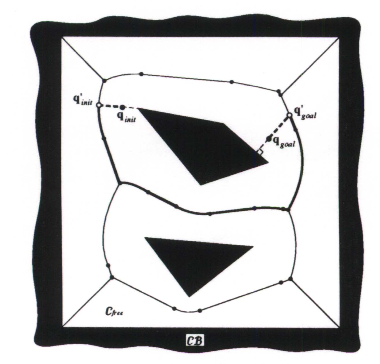
        There are various types of roadmaps, including the visibility graph, the Voronoi diagram, the freeway net, and the silhouette.  One of the earliest path planning methods was the visibility graph method, explored by NJ Nilsson as early as 1969.  A visibility graph is shown below.   The shaded areas represent obstacles.  The solid lines are the edges of the graph and connect the vertices of the obstacles.  The dotted lines connect the beginning and end configurations with the roadmap.
 

        The figure below shows a Voronoi diagram in a configuration space with a polygonal C-obstacle region.  This diagram is a planar network of line segments and parabolic curves, which are the set of points equidistant from at least two obstacles.  The path generated by this method keeps the robot as far away from the obstacles as possible, unlike the visibility graph.
 

        The basic idea behind this method is that a path between the initial configuration and the goal configuration can be determined by subdividing the free space of the robot's configuration into smaller regions called cells.  After this decomposition, a connectivity graph, as shown below, is constructed according to the adjacency relationships between the cells, where the nodes represent the cells in the free space, and the links between the nodes show that the corresponding cells are adjacent to each other.  From this connectivity graph, a continuous path, or channel, can be determined by simply following adjacent free cells from the initial point to the goal point.  These steps are illustrated below using both an exact cell decomposition method and an approximate cell decomposition method.
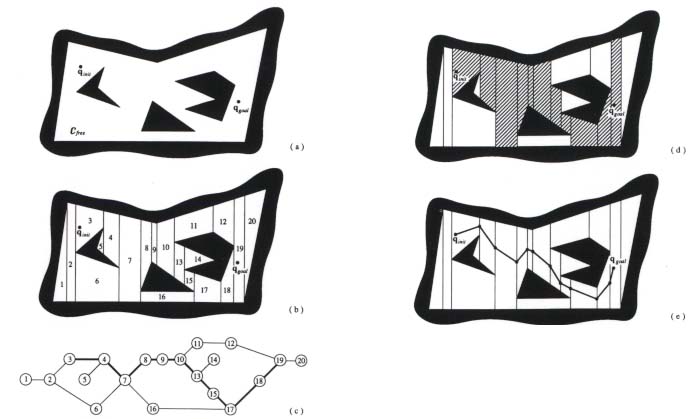
Exact Cell Decomposition
        The first step in this type of cell decomposition is to decompose the free space, which is bounded both externally and internally by polygons, into trapezoidal and triangular cells by simply drawing parallel line segments from each vertex of each interior polygon in the configuration space to the exterior boundary.  Then each cell is numbered and represented as a node in the connectivity graph.  Nodes that are adjacent in the configuration space are linked in the connectivity graph.  A path in this graph corresponds to a channel in free space, which is illustrated by the sequence of striped cells.  This channel is then translated into a free path by connecting the initial configuration to the goal configuration through the midpoints of the intersections of the adjacent cells in the channel.
 

Approximate Cell Decomposition

    This approach to cell decomposition is different because it uses a recursive method to continue subdividing the cells until one of the following scenarios occurs:

• Each cell lies either completely in free space or completely in the C-obstacle region
• An arbitrary limit resolution is reached.

        Both exact cell decomposition methods and approximate cell decomposition methods have advantages and disadvantages.  The former are guaranteed to be complete, meaning that if a free path exists, exact cell decomposition will find it; however, the trade-off for this accuracy is a more difficult mathematical process.  Approximate cell decomposition is less involved, but can yield similar, if not exactly the same, results as exact cell decomposition.

        The potential field method involves modeling the robot as a particle moving under the influence of a potential field that is determined by the set of obstacles and the target destination.  This method is usually very efficient because at any moment the motion of the robot is determined by the potential field at its location.  Thus, the only computed information has direct relevance to the robot's motion and no computational power is wasted.  It is also a powerful method because it easily yields itself to extensions.  For example, since potential fields are additive, adding a new obstacle is easy because the field for that obstacle can be simply added to the old one.
        The method's only major drawback is the existence of local minima.  Because the potential field approach is a local rather than a global method (it only considers the immediate best course of action), the robot can get "stuck" in a local minimum of the potential field function rather than heading towards the global minimum, which is the target destination.  This is frequently resolved by coupling the method with techniques to escape local minima, or by constructing potential field functions that contain no local minima.