Proximal Gradient Descent

Something I quickly learned during my internships is that regular 'ole stochastic gradient descent often doesn't cut it in the real world. Data are too big and too noisy. The models are too refined, too complex. Loss functions are non-convex. Sadness. Fortunately, there's a whole bunch of tricks statisticians have cooked up to let us train on even the gnarliest of error surfaces. Proximal gradient descent (PGD) is one such method.

Ok. Let's backtrack a bit and start from the very top. PGD falls into a broader category of algorithms that fit statistical models to data. This fitting usually requires some sort of optimization. In a perfect world the function we are trying to optimize is convex, differentiable, and unconstrained. This means all we would need to do is basic gradient descent.

In many real world applications, though, we don't have this luxury. A great example is the class of models with L1 regularization schemes like Lasso regression. This regularization method is an effective promoter of sparsity but it results in a loss function that is non-differentiable (aka it has kinks). This introduces a whole bunch of problems. For example, we might not always be able to compute a gradient to descent. Proximal gradient descent is a way of getting around this.

As an aside, you may have noticed that I keep on switching between "PGD" and "proximal gradient descent". No consistancy. It seems like the literature vdoes the same thing, though. I think in both cases it's because we have a tendancy to gravitate towards compressed 3-letter acronyms but can't resist writing something that sounds as badass and intense as "proximal gradient descent".

Some Definitions

The method makes use of two mathematical tools you may not have heard of already. Lets talk about them.

1) Sub-Gradients

sub-gradients are a generalization of the concept of the gradient, which can be applied to non-differentiable functions.

First, let's visualize what the gradient of a convex, differentiable function looks like. These functions look like the mouth of a smiley face. The gradient of such a function is like a line which touches the curve at only one point. Note that if this is going to be true, the entire rest of the function is held above this line. Ok. That was painless.

Let's go on to convex non-differentiable functions. These are like smiley mouths (wow "mouths" is a super weird looking word) with at least one kink, and they have sub-gradients instead of gradients. Sub-gradients are sets of vectors. Each vector in this set is kind of like a gradient. They touch at only one point and the entire function is held above them. This means that the only element in the sub-gradient IS the gradient at all the smooth, curvey parts of our function. At the kinks, though, the sub-gradient is the set of all lines which are below the function. Subgradient at x0. Simple, right?

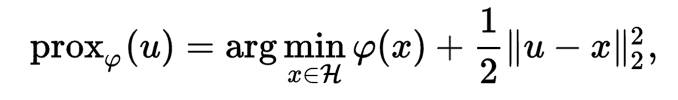
2) Proximal Operators

The proximal operator takes a point in a space (x) and returns another point (x'). It is parameterized by a function (f) and a scalar (g).

x' is chosen because it both minimizes f and is close to x (in the L2 sense). The tradeoff between minimizing f and staying close to x is determined by g. Yeah yeah the notation is not what I used but I know you love formulas soo take it or leave it.

Optimality Conditions

At the minimum of a differentiable function the gradient must be zero. This is because if it wasn't zero, we could just move in the direction of -gradient(f).

For non-differentiable convex functions, this optimality contidion isn't helpful because the minimum might be a kink where you can't differentiate.

Good thing we have our old friend the sub-gradient! Even if the the minimum point $x$ is a kink, 0 must be in the set of sub gradient's at $x$.

Algorithm Overview

Basically it works like this:

1. Break f into two parts: g (the differentiable part) and h (the non-differentiable part).
2. Take a step along the gradient of g to minimize that part of the function.
3. Use the proximal operator to take another step that reduces h while staying close to the point selected by (2)
4. Repeat (2) and (3) until the optimality condition is met.

Python Pseudo(ish)code

import Math


def proximal_descent(g, g_prime, h_prox, x0, iterations = 1000, gamma = 1.0, epsilon = 1e-4):
    """
    minimizes a non-differentiable function f(x) = g(x) + h(x)
    PARAMS
    g: function
        g(x), the differentiable part of f
    
    g_prime: function
        g'(x) aka the gradient of g
        returns the direction of steepest increase along g
    h_prox: function
        h_prox(x, gamma) returns proximal operator of h at x using gamma as a distance weighting param
        h_prox gives a new x' which is a tradeoff of reducing h and staying close to x
    x0: vector
        initial stariting point
    iterations: self explanitory
    gamma: step size
    
    epsilon: self explanitory
    RETURNS
    x* = argmin_x { f(x) } if x* is reachable in the given num iterations. else None
    """
    # initialize current guess at x0
    xk = x0
    gk = g(xk)

    for _ in range(iterations):
        xk_old = xk
        # compute gradient for differentiable  part of f
        gk_gradient = g_prime(xk)
        # take gradient step to reduce g(x)
        xk_gradient = xk - gamma * gk_gradient
        # proximal update to reduce h(x) but stay close to xk_gradient
        xk = h_prox(xk_gradient, gamma)

        if Math.abs(xk - xk_old) < epsilon:
            return xk

    return None